Fitting a spline nonlinearity in a Poisson model

I was talking to Jeremy Freeman at CSHL and he asked about an easy way to fit a spline nonlinearity in a Poisson regression model. Recall that with the canonical exponential nonlinearity, we have the following setup:

$\eta = Xw \newline r = \exp(\eta) \newline y \sim Poisson(r)$

And the negative log-likelihood is given by:

$\sum_i y_i \log(r_i) - r_i$

Start by fitting w by maximum likelihood. Compute $\eta$ . Then you can do one of two simple things to fit the output nonlinearity with a spline. Choice 1 is to set 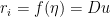$r_i = f(\eta) = Du$ , where D is the basis matrix for the spline, and u is a set of weights. You want to use fmincon with A equal to the negative of the basis matrix for the spline evaluated at equispaced points in the range of the spline and B set to a vector of small equal negative values (say -.0001).

A second option is to set $r_i = \exp(f(\eta_i)) = \exp(Du)$ . In that case, the model reduces to Poisson regression and can be fit through unconstrained optimization.

June 25, 2012

6 responses to “Fitting a spline nonlinearity in a Poisson model”

xcorr says:

June 25, 2012 at 10:36 am

I just talked to Jeremy and he said that what he does on a regular basis is use the a log(1+exp(x)) nonlinearity during the model fitting stage and at the very end he fits a spline (he doesn’t refit the other model parameters after fitting the spline). That seems to me like a reasonable way of balancing the requirement of convexity/log-concavity with the use of a flexible output nonlinearity.

Reply
- jpillow says:
  
  June 25, 2012 at 2:43 pm
  
  I think the only caveat to Jeremy’s approach is that I’ve found you can get very different fits with different transfer functions — exp vs. log(1+exp(x)) — when fitting GLM. Both functions decay exponentially on the left tail, but log(1+exp(x)) grows only linearly on the right – that can be a good thing if it’s a nonlinear transfer function for a cubic spline (giving you x^3 instead of e^(x^3) growth), but may not be great for standard GLM. (So Patrick: your choice of functions for extrapolation on left and right sides map perfectly onto this function).
  
  In general, it’s a data-dependent question, so I think worth trying a few different choices of transfer function (“inverse link function” in standard GLM terminology). For the retinal data from our 2008 paper, “exp” was much better than log(1+exp(x)), but best overall was log(1+exp(x))^p, for p around 3. (But best p varied across cells and differed a bit for OFF vs. ON).
  
  Reply
  - xcorr says:
    
    June 25, 2012 at 3:44 pm
    
    Right, but $a \log(1+\exp(x-log(a))) \approx \exp(x)$ for large a, and $a \log(1+\exp(x/a)) \approx \mbox{thresh}(x)$ for small a. So you probably use 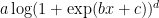$a \log(1+\exp(bx+c))^d$ as a one-size-fits-all output nonlinearity, and it would cover threshold functions, power law nonlinearities, linear, exponential, etc. This way you wouldn’t need to do separate fits for each nonlinearity you want to consider.
  - jpillow says:
    
    June 26, 2012 at 11:43 am
    
    nice!
xcorr says:

June 25, 2012 at 10:28 am

Excellent points. Indeed, Dan Butts told me that he’s been having a lot of success with $a \log(1+exp(x))$ . I’ve done a version of the spline nonlinearity that follows the convex/log-concave conditions and that gives a range of nonlinearities that is very well fit by the $a \log(1+exp(x))$ family. In that version I extrapolated outside the range with exp(x) on the left-hand side and linear on the right-hand side with the natural continuity conditions.

Reply
jpillow says:

June 25, 2012 at 1:16 am

Or, more generally: pick any function g whose output is strictly positive. Then set r = g(D\mu). If g is convex and log-concave, then the log-likelihood is log-concave in \mu for spine basis matrix D (Paninski 2004 Network).

Our Poisson-GLM implementation (http://pillowlab.cps.utexas.edu/code_GLM.html) contains one implementation of this, but only for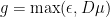 $g = \max(\epsilon,D\mu)$ . i.e., linear half-wave rectified above a small constant. I’ve recently found $g = \log(1+\exp(x))$ is better, since it also satisfies the conditions above, but has continuous derivatives of all orders. (I have yet to add this to the implementation, but it’s on my list).

Final thought: g = exp may be a bad choice if you ever need to extrapolate beyond the range of the stimuli used for training, since you’ll effectively have growth or decay of exp(+/- x^3) for a cubic-spline basis.

Reply