Using Non-negative matrix factorization instead of SVD

Sujay, a labmate of mine came to me with an interesting analysis problem. He’s looking at perisaccadic changes in receptive fields in V4. The saccade-triggered receptive fields shows two activations: an initial one at the pre-saccadic location, and a later one at the remapped location. Basically, the activation looks like this:

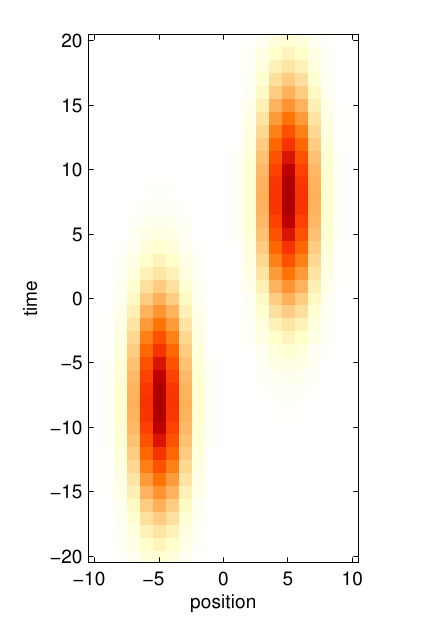
He asked if there’s a way to isolate these two components. The perisaccadic receptive field, viewed as a matrix with one dimension corresponding to time and the other to space, is low-rank, , with U and V containing two columns.

At first sight, the natural tool to estimate such a low-rank decomposition is the SVD; however, SVD doesn’t find the right kind of spatio-temporal decomposition. As shown below, it extracts a mean and a difference component:

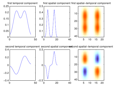
What we’d like instead is to extract two spatio-temporal components which are localized. Unlike an SVD type decomposition, we make no assumption that the components are orthogonal. What can we assume instead?

Well, we might want to assume that the components are sparse, localized in space and time, unimodal, etc. But really the simplest assumption that does the trick is to simply assume that each component is positive. Running Matlab’s non-negative matrix factorization (NNMF) implementation on this example returns the kind of decomposition we were looking for:

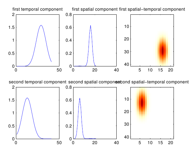
NNMF is extremely fast and takes only a couple of iterations to converge in this type of problem.

Of course, with noisy data it doesn’t work as well, but it can be used to kick-start a fancier decomposition. For example, you can assume that each component of the RF is localized; such a model is can be fit with a straightforward extension of the low-rank ALD method in Park & Pillow (2013).

I’m waiting on Mijung for the code, but in the meantime I’m using an iterative approximation to low-rank ALD via projecting out every other component and running ALD on the residual. It works really well. Here’s a PDF with code and more examples.

Signed tensor factorization for multilinear receptive fields

I thought I had simply found a neat trick for a very peculiar estimation problem, but then I ran into a related problem a few weeks later. As it turns out, there are many situations in neural data analysis where NNMF and its extensions are the right tool for the job; it’s an under-exploited tool.

The problem is the following: I’m estimating receptive fields in V2 with some new methods and consistently finding tuned, off-centered suppression. Reviewers are often wary of fancy methods – with reason! – so I thought it’d be nice to show that the off-centered suppression is visible, if noisy, in minimally processed data.

Running normalized spike-triggered averaging in a rectified complex Gabor pyramid basis, it’s clear in many neurons that there are excitatory and suppressive components. Here’s an example where the cell appears excited by high contrast on the right and suppressed by high contrast on the left:

The question is, how can you isolate these two components without making strong assumptions about the shape of the receptive fields? If the receptive field is defined as a tensor , where s is space, o is orientation, and t is time lag, then we can assume that it is generated by the sum of two components, an excitatory one and a suppressive one. Let’s assume that each component is a rank-1 tensor; then we have:

If the sign was positive instead of negative we could use non-negative tensor factorization, an extension of NNMF to tensors. Instead, we can use what you might call signed tensor factorization, where the sign of each component is user specified. Algorithmically, you can simply multiply one of the components by -1 at the right time. Here’s what I get applying it to the example above:

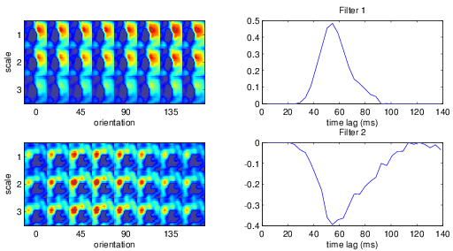
Interestingly, the suppressive component appears to have a slightly longer time course than the excitatory one. Here’s another example:

This time, the time course is more similar, but the tuning to orientation is quite different. Once we have this decomposition in hand, we can feed it as start parameters to a multilinear GLM to obtain a generative model for the data; this corrects for the strong correlations in the stimulus when represented in a Gabor pyramid. Here is the multilinear receptive field estimated via a GLM with a sparseness prior on the spatial weights, Von Mises orientation tuning, non-negative spatial frequency tuning, and smooth temporal filter:

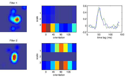
Here you can pretty clearly that the second component is slightly off-centered (to the left), tuned to an orthogonal orientation to the preferred orientation of the first, and also slightly delayed and longer lasting.

In case you’re wondering, a model with two components is not much better than one with only a single component at predicting the spikes; that’s because there’s internal nonlinearities in both the excitatory and inhibitory components. So you still need the shared deep neural net magic  model™, but at least now you can demonstrate that one of the prominent things it finds – off-centered inhibition – is not an artifact of its complex internals.

Here’s some example code to do signed tensor factorization:

function [ws,normbest] = signedtf(M,signs,nreps)
    %Signed matrix factorization
    if nargin < 3
        nreps = 10;
    end
    dnorms = zeros(nreps,1);
    Ws = cell(nreps,1);
    for ii = 1:nreps
        [Ws{ii},dnorms(ii)] = signedtfsub(M,signs);
    end
    [normbest,themin] = min(dnorms);
    ws = Ws{themin};
end

function [ws,normbest] = signedtfsub(M,signs)
    %Signed matrix factorization
    dispnum = 3;
    signs = signs(:);
    nm = numel(M);
    ndim = ndims(M);

    %Create initial guesses
    ws = cell(ndim,1);
    for ii = 1:ndim
        if ii < ndim
            ws{ii} = rand(size(M,ii),length(signs));
        else
            ws{ii} = bsxfun(@times,signs',rand(size(M,ii),length(signs)));
        end
    end
    
    maxiter = 100;
    dispfmt = '%7d\t%8d\t%12g\n';
    repnum = 1;
    tolfun = 1e-4;


    for j=1:maxiter
        % Alternating least squares
        
        for ii = 1:ndim
            %shift dimensions such that the target dimension is first
            Mi = shiftdim(M,ii-1);
            Mi = reshape(Mi,size(Mi,1),numel(Mi)/size(Mi,1));
            
            %Compute Hi
            Hi = compute_prods(ws,ii);
            if ii < ndim
                ws{ii} = max(Mi/Hi,0);
            else
                ws{ii} = bsxfun(@times,max(bsxfun(@times,Mi/Hi,signs'),0),signs');
            end
        end
        
        %Reconstruct the full product
        Hp = reconstructM(ws);

        % Get norm of difference and max change in factors
        d = M - Hp;
        d = d(:);
        dnorm = sqrt(sum(sum(d.^2))/nm);

        % Check for convergence
        if j>1
            if dnorm0-dnorm <= tolfun*max(1,dnorm0)
                break;
            elseif j==maxiter
                break
            end
        end

        if dispnum>2 % 'iter'
           fprintf(dispfmt,repnum,j,dnorm);
        end

        % Remember previous iteration results
        dnorm0 = dnorm;
    end

    normbest = dnorm0;
    
    if dispnum>1   % 'final' or 'iter'
        fprintf(dispfmt,repnum,j,dnorm);
    end
end

function as = reconstructM(ws)
    as = ones(1,size(ws{1},2));
    szs = zeros(1,size(ws{1},2));
    for jj = 1:length(ws)
        theidx = jj;
        for kk = 1:size(ws{1},2)
            theM = as(:,kk)*ws{theidx}(:,kk)';
            if kk == 1
                allM = zeros(numel(theM),size(ws{1},2));
            end
            allM(:,kk) = theM(:);
        end
        as = allM;
        szs(jj) = size(ws{jj},1);
    end
    as = reshape(sum(as,2),szs);
end
function as = compute_prods(ws,ii)
    as = ones(1,size(ws{1},2));
    for jj = 1:length(ws)-1
        theidx = mod(jj+ii-1,length(ws))+1;
        for kk = 1:size(ws{1},2)
            theM = as(:,kk)*ws{theidx}(:,kk)';
            if kk == 1
                allM = zeros(numel(theM),size(ws{1},2));
            end
            allM(:,kk) = theM(:);
        end
        as = allM;
    end
    as = as';
end