Reverse correlation: linearizing black-box functions

Reverse correlation is a tried-and-tested nonlinear systems identification method to understand biological neurons. The idea is to open the black box that is a biological neuron by using random stimuli to probe how the neuron responds. We present a series of random stimuli to a sensory neuron. By averaging those that generated a response, we obtain the spike-triggered average. The spike-triggered average is equal to the weights of a linear filter that approximates the response of a neuron. Under this linearity assumption, it is also a neuron’s preferred stimulus.

Reverse correlation in a nutshell. Source: Wikipedia.

Reverse correlation has fallen out of favour as people have graduated to more complex models (e.g. GLMs and deep nets) with more complex stimuli (natural scenes) to probe brain representations. However, the machinery underlying reverse correlation is making somewhat of an unexpected comeback in different corners of machine learning. This is something that I’m sure will surprise many machine learning people as well as neuroscientists. Digging deeper into these subfields yields some insights on improvements in nonlinear systems identification that we can take back to computational neuroscience. In this article, I discuss two of these ideas:

evolution strategies, which are black-box optimization methods
locally interpretable models, which are linearization models to open up black box models like deep neural nets

Before I dig into these methods, let’s dig into the theory behind reverse correlation so we can understand its deep structure.

The theory behind reverse correlation

Reverse correlation seemed pretty magical when I first encountered it! Put noise into a system, measure responses – out comes the kernel (?!). I ended up writing my PhD thesis on systems identification, so you’d think that by the time I graduated my thinking on this was solidified. In the years since, I’ve found that reverse correlation is actually pretty darn subtle, and I’ve developed a new appreciation for all the subtle aspects of the technique.

There’s a good exposition of the ideas behind reverse correlation in Franz & Schölkopf (2006). Let’s say that we are trying to characterize a nonlinear system that receives $N$ real inputs and outputs a noisy scalar $y$ :

$\mathbb E [y|x] = f(\bold x) \newline \text{where } \bold x \in \mathbb R^N$

Then, under certain regularity conditions, we can write the mean response function of the system $f(\bold x)$ as a polynomial expansion, the Volterra expansion:

$f(\bold x) \approx h_0 + (\bold x - \bold x_0)^T \cdot h_1 + (\bold x - \bold x_0)^T h_2 (\bold x - \bold x_0) + \ldots$

Note that the kernels $h_i$ have increasing order: $h_0$ is a scalar, $h_1$ a vector, $h_2$ a matrix, $h_3$ a three-index tensor, etc. The form of the expansion is similar to a Taylor expansion, and it’s tempting to identify the two.

Misconception: the Volterra expansion is a Taylor expansion

The Volterra expansion is more general than a Taylor expansion: a Taylor expansion requires well-defined derivatives to every order, while a Volterra expansion does not. For example, the function $f(x) = \exp(-1/x^2)$ has 0 derivatives everywhere. Hence, its Taylor expansion around 0 is exactly 0. However, it has a perfectly good non-null Volterra expansion, which can be found through polynomial regression. Here’s a notebook that shows you how it’s done.

Approximating a function with a null Taylor series with polynomials.

This subtle difference might seem like some nit-picking, but in practice, it is very important: discontinuous functions and stochastic functions can both be approximated with Volterra series. Biological Neurons are both stochastic and have potentially very sharp nonlinearities, yet we can still approximate them using a Volterra expansion.

The Wiener expansion is an orthogonalized version of the Volterra expansion.

To estimate the coefficients of the Volterra expansion, conventional reverse correlation first rearranges the Volterra expansion into an equivalent series of functionals, the Wiener expansion:

$f(\bold x) = \sum_i G_i[\bold x]$

And imposes that these functionals are orthogonal to each other:

$\mathbb E_D[G_i(x)G_j(x)] = 0 \text{ for } i \ne j$

Here $D$ is the data distribution. Orthogonality is imposed via a Gram-Schmidt orthogonalization process:

Set $G_0$ to the output of the Volterra kernel of order 0
Set $G_1$ to the output of the Volterra kernel of order 1, and back-project $G_0$ from $G_1$ to make $G_1$ orthogonal to $G_0$
Set $G_2$ to the output of the Volterra kernel of order 2, and back-project $G_0$ and $G_1$ from $G_2$ to make $G_2$ orthogonal to both, etc.

This is the itty-bitty subtle bit: it turns out that the expectations of every order are straightforward to calculate when the data distribution $D$ is normal. The 0’th order and 1st order functionals are simply the constant and linear Volterra kernels. The 2nd order functional is the quadratic kernel minus a correction for the diagonal terms of the kernel, since the square of a normally-distributed variable distribution has a mean equal to the square of the standard deviation, $\mathbb E[x^2] = \sigma^2$ . Thus:

$G_0 = k_0 \newline G_1 = (x - x_0)^T k_1 \newline G_2 = (x - x_0)^T k_2 (x - x_0) - \sigma^2 \sum_j k_2^{jj}\newline$

Since each functional are orthogonal over the data distribution, we can easily calculate them using an iterative procedure:

Estimate the Wiener kernel $k_0$ from the measured response $y$
Project the 0’th order functional out of $y$ to obtain $y_{res}$
Estimate the Wiener kernel $k_1$ from the residual $y_{res}$ , etc.

Estimating Wiener series with white noise means finding estimates that minimize sum-of-squares between prediction and measurement over the stimulus ensemble. We use a few shortcuts enabled by properties of white noise.

What does estimate mean in this context? Least-squares! To estimate the zero-order kernel, we have:

$\hat k_0 = \arg \min_{k_0} \sum(y - k_0)^2 = \bar y$

For the first-order kernel:

$\hat k_1 = \arg \min_{k_1} \sum(y - \bar y - (x - x_0)^T k_1 )^2 \newline = ((x - x_0)^T (x-x_0))^{-1} (x-x_0)^T (y - \bar y) \newline \approx \frac{1}{N \sigma^2} (x-x_0)^T (y - \bar y)$

Here the approximate sign comes from the fact that with normally distributed data, $(x - x_0)^T (x-x_0) \approx N\sigma^2 I$ . The second order kernel is a little more tricky. We first define $r = y - \bar y - (x - x_0)^T$ . Then:

$k_2 = \arg \min_{k_2} \sum \left(r - (x - x_0)^T k_2 (x - x_0) + \sigma^2 \sum_j k_2^{jj} \right)^2 \newline = \text{unstack}((D^T D)^{-1} D^T r) \newline$

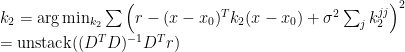
The columns of the matrix $D$ is composed of all the cross-products $x_i x_j - \delta_{ij} \sigma^2$ for $i \ge j$ . The operator $\text{unstack}$ takes this linear representation of the coefficients and transforms them into a matrix. Here again, we find that for normally distributed inputs, the non-diagonal terms in the covariance matrix $D^TD$ have an expected value of zero. The inverse of the diagonal is a bit more tricky to calculate, but a little bit of grinding shows that we pick up a scalar factor $\frac{1}{2!\sigma^{4}}$ . In fact, we can show that the estimate of the kernels can be written as:

$k_i(j_1, j_2, \ldots j_i) = \frac{1}{i!\sigma^{2i}N} [y - \sum_{m=0}^{i-1} G_m(\mathbf x)] x_{j_1} x_{j_2} \ldots x_{j_i}$

Where $G_j$ are the orthogonalized Wiener functionals (equation 2, Korenberg et al. 1988). Notice the $i!$ factors, which look an awful lot like a Taylor expansion. This formula actually works! Here’s a notebook to show you how it’s done for a second order Wiener expansion.

Is your head spinning yet? Mine sure was! Grinding through the kernels one by one makes a few things clear:

Wiener-Volterra analysis isn’t magic. It’s orthogonal polynomial regression estimated through least-squares, with approximations that are enabled by the use of a very special distribution of the inputs, the normal distribution. This means that expectations of different moments can be analytically calculated.
The Wiener kernel definitions change when you change the distribution of the input. This is because orthogonalization is dependent on the input distribution.
The easy estimation of the kernels via backprojection and simple multiplication with cross-products of the inputs is lost when the input distribution is not normal.

The special properties of white noise were very important technically in 1958 when the series was proposed: the kernels could be estimated with very minimal computing resources. A memoryless accumulator is sufficient. Today, we’re no longer bound by these limitations, and we can do Wiener-Volterra analysis in a much wider range of contexts. Casting Wiener-Volterra analysis as polynomial regression fit via least-squares immediately opens up many extensions:

Finding better estimates via the minimum variance unbiased estimator, that is, maximum likelihood
Finding better estimates by better modeling the noise, for example, taking into account the Poisson nature of neural noise
Generalizing to non-normally distributed ensembles of inputs, again using maximum likelihood
Using alternative expansions, for example, cascades of linear-nonlinear filters (i.e. deep nets), fit with stochastic gradient descent

Remarkably, some of the ideas behind Wiener-Volterra theory – local polynomial expansion, probing stimuli at random – have made their way into far-flung machine learning methods. Let’s take a look.

Evolution strategies (ES)

Evolution strategies (ES) are a family of black-box, gradient-free optimizers for potentially non-differentiable functions. At the heart of most optimizers over continuous variables is the computation of the gradient. If the gradient is unaccessible because of discontinuities, or because it is very expensive to calculate, we can obtain a smoothed gradient via the ES method.

The setup is quite clever. We have a function $f$ that we are trying to optimize. Instead of computing its derivative $\nabla f(z)$ directly, we compute the derivative of the expectation of the function, $\mathbb \nabla \mathbb E_\pi[f(z)]$ in a local neighborhood $\pi(\theta, z)$ . Think of this expectation as a smoothed derivative.

To compute the expected value, we expand it via its definition, and obtain:

$\nabla_\theta \mathbb E_\pi(z, \theta)[f(z)] = \nabla \int \pi(z, \theta) f(z) dz \newline = \int \nabla \pi(z, \theta) f(z) dz \newline = \int \nabla \log \pi(z, \theta) \pi(z, \theta) f(z) dz$

The last equality, which is also called the log-derivative trick, is derived from:

$\nabla \log \pi(z,\theta) = \frac{\nabla \pi(z, \theta)}{\pi(z, \theta)}$

A neighbourhood which is often used in practice is the isotropic Gaussian centered at $\mu$ with a standard deviation $\sigma$. If we take a Monte Carlo estimate of the expectation, we find an approximation for the gradient as:

$\nabla \mathbb E[f] \approx \frac{1}{N} \sum_{1}^N \nabla_\mu \log N(\mu, \sigma^2) \newline = \frac{1}{N} \sum_{1}^N \frac{1}{\sigma^2} (z-\mu) f(z)$

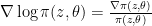
Notice this remarkable equation: this is exactly the response-triggered average with an isotropic gaussian stimulus ensemble. This reveals an unexpected link between reverse correlation and optimization: we can view reverse correlation as estimating an approximate gradient of the response function of a neuron.

The response-triggered average tells us how we should change a stimulus locally to increase the response of the system.

Taking ES to reverse correlation

From the OpenAI blog.

The unexpected link between reverse correlation and optimization opens up a lot of different avenues. For instance, we could adapt ES to maximize the response of a neuron in a closed-loop fashion. This strategy has the advantage of being trivial to compute and highly intuitive (i.e. no complaints from reviewer 2 about the method being inscrutable).

ES is also embarrassingly parallel, which has been used to good effect in the context of reinforcement learning – OpenAI showcased ES with 1024 parallel evaluations. We could consider evaluating the gradient of a neuron’s response function in parallel with several other neurons – perhaps in a different animal, in a different lab – and optimize for a stimulus that maximizes the sum of the responses. Indeed, we don’t have to focus on maximizing just the mean response of a neuron: we can maximize the diversity of responses, their dimensionality, etc. This works as long as the metric that we’re measuring is a scalar function of the measured responses.

ES comes in a variety of different flavours that aim to increase the efficiency of the method. Two of the most popular variants are:

CMA-ES (Covariance-matrix-adaptation). This takes the derivative of the neighborhood with respect to the covariance of the normal distribution, in addition to its mean. Thus, the covariance stimulus ensemble is tweaked to capture the largest dimensions of descent.
NES (Natural evolution strategies). This uses natural gradients rather than gradients, which naturally deals with rescaling of the axes.

Both of these more efficient variants could be applied to find preferred stimuli in a population of neurons.

Finally, because the ES objective is a Monte Carlo estimate, we can import many of the tricks from the variance reduction literature to increase the efficiency of reverse correlation. For example, we can use control variates or use stratified sampling strategies. My favourite trick to increase the efficiency of estimation: pairing every stimulus with its negative. With this trick, the mean of the realized stimulus ensemble is exactly the mean of the distribution. This antithetic sampling can, in some circumstances, increase the efficiency of the estimation of the preferred stimulus.

Locally interpretable models

There’s another area where the ideas underlying reverse correlation have recently come together: locally interpretable models. Suppose that we have a complex black-box model that we are trying to better understand. This black box model can be, for example, a deep neural network. We can locally approximate this complex function with a simpler, local expansion. This local explanation does not capture all the subtleties of the model, but it can reveal insights that are useful for humans that want to understand the model.

Black-box models are good for predictions by machines. White-box models are good for understanding by humans. LIME transforms black-box models into locally white-box models.

From the LIME paper, Ribeiro et al. 2016.

In general, we try to find a model $g$ which approximates a complex function $f$ according to a weight window $\pi$ :

$\arg \min_{g\in G} L(f, g, \pi) + \Omega(g)$

Here $L$ is a loss function and $\Omega(g)$ captures the complexity of $g$ . In LIME, or locally interpretable model explanations, the authors suggest to use a Gaussian-shaped neighborhood around an anchor $a$ , and a sum-of-squares loss, leading to the weighted loss:

$L = \sum_i \exp \left(-\frac{||x_i - a||^2}{\sigma^2} \right) (f(x_i) - g(x_i)) ^ 2$

Several choices are possible for $\Omega(g)$ . For example, we may privilege functions that focus on few input dimensions; we can impose that $g$ is sparse in parameter space using an L1 penalty as $\Omega(g)$ . The model class $G$ can be anything that is “easy to interpret” for humans. This could mean:

a GAM
a decision tree
a linear model

If we choose no penalty for complexity and choose a linear model class, our model and error function is equivalent to reverse correlation and evolutionary strategies. This highlight something that’s underappreciated about reverse correlation:

The spike-triggered average is a simplified, locally valid explanation for how a neuron works. While complex models like deep nets can capture more of the variance in the data, the goal in reverse correlation is different: explaining neurons to humans.

Taking LIME to reverse correlation

An underappreciated fact about reverse correlation is that the size of the neighbourhood around which we’re linearizing is arbitrary and that different neighbourhoods will lead to different estimates.

Many articles have documented that receptive fields appear to change with changing stimulus ensembles, for example natural vs. artificial stimuli. However, this has been explained in terms of a special, adaptive response of neurons to natural image statistics; for instance, that they increase the degree of feedforward inhibition they receive. In fact, the same phenomenon could happen simply because we’re measuring a nonlinear function, so that its locally linear expansion depends on the stimulus ensemble.

Many of the parameters of the probing distribution are arbitrary:

the size of the neighborhood (big vs. small)
the shape of the neighborhood (isotropic Gaussian vs. non-isotropic vs. natural stimuli)
the center of the neighborhood (gray image or another reference)

Some of the most interesting applications of nonlinear systems identification have manipulated each of these factors. For example, by shifting the center of the neighbourhood to an appropriate anchor point, we can locally linearize quadratic responses (i.e. complex cells) by choosing an appropriate anchor point. This is the idea behind Movshon et al. (1978), where the line weighting function of a complex cell is found by using another line in the center as an anchor:

From Movshon et al. 1978.

There are some other excellent nuggets in the LIME paper that could serve us well. For instance, they suggest using a maximally diverse ensemble of examples (SP-LIME) to illustrate the functioning of the models to humans. A similar idea was used in Cadena et al. (2018) to visualize diverse features that triggered large responses in early stages of a deep neural net around an anchor point (invariant or equivariant features).

Finally, we can have our cake and eat it too: we can fit very complex models of neurons that explain much of the variance in sensory systems using deep nets, and visualize how these models work using locally linear explanations. It sounds a little silly to fit a model to a model, but it’s a technique that has been used fruitfully both to explain sensory neurons and to compress neural networks.

Conclusions

Both ES and LIME use local linearization strategies similar to reverse correlation to explain complex black box function. From ES, we learn that the reverse correlation estimate gives us a local approximation for the gradient, which can be used as a starting point for closed-loop experiments. From LIME, we see that we can perform reverse correlation centered around different neighbourhoods, yielding different results. By following these new research trends in machine learning, we can find innovative ways of opening the black boxes that are biological neurons.

xcorr: AI & neuro