I’ve used OpenBUGS for Gibbs sampling in the past, and while it’s a powerful piece of software, I hate OpenBUGS’ GUI, especially since it runs only on Windows. JAGS is an alternative Gibbs sampling program that uses an OpenBUGS-like syntax and runs on the command line. You can call JAGS in R through the rjags package and analyze the convergence of the MCMC chains through the coda package. It works beautifully, especially with RKWard, an alternative GUI for R that runs on Linux that is quite satisfying to use.

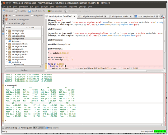
While its features do not rival that of Matlab — it doesn’t support debugging, for example –, it certainly eases you into the R language with features like syntax highlighting, inline help, and menus to perform common statistical analyses. Here’s a screenshot:

With RKWard and this Matlab to R cheat sheet, you can get started doing Gibbs sampling painlessly in minutes.

Installation

You can install JAGS and RKWard in Ubuntu at the terminal:

sudo apt-get install jags rkward

Then after opening RKWard you can install the “coda” and “rjags” packages through the Settings > Configure Packages menu, or by running the R command install.packages().

Simple example

Here’s a simple example taken from chapter 5 of Bayesian Data Analysis by Gelman et al. The problem is to determine whether different SAT training programs have a positive effect on SAT scores. We are given the summary statistics of the distribution of changes in SAT scores following training in 8 schools (mean and standard deviation), and they are quite noisy. Because of this noise, we might want to pool the scores from the different schools together to determine the overall effect of training, despite the fact that the schools used different programs. On the other hand, if we want to determine the effect in any individual school we can’t pool the results, and that means individual inference will be very noisy.

Gelman proposes that instead of either pooling everything together or doing no pooling at all, we should use a hierarchical model in which the mean training effect is taken from a distribution with mean 0, a school’s individual effect is taken from a distribution with mean equal to the mean training effect, and the observed scores are taken from distributions centered around individual effects. By tweaking the standard deviation (sigma) of the distribution of the school’s individual effects, we can obtain the equivalent of no pooling (sigma -> Infinity) or full pooling (sigma -> 0), or something in between.

Defining the model with JAGS syntax

The model is defined in JAGS syntax, which is similar to that of OpenBUGS, as:

model {
for(i in 1:N) {
schoolmean[i] ~ dnorm(mu,itau)
thes[i] <- 1/pow(sigma[i],2)
schoolobs[i] ~ dnorm(schoolmean[i],thes[i])
}

mu ~ dnorm(0,alpha)
alpha <- .01
itau   ~ dgamma(1e-3,pow(15,2)*1e-3)
tau <- pow(1/itau,1/2)
}

This model can be saved as ~/Documents/ch5gelman.model.

Running the model in R

We can write the data (Table 5.2 in Gelman) in R syntax as:

sigma     <- c(15,10,16,11, 9,11,10,18)
schoolobs <- c(28,8, -3, 7,-1, 1,18,12)

To run the model, we include rjags and coda through the library command, and write:

library("rjags")
library("coda")
jagresult <- jags.model('~/Documents/ch5gelman.model',data=list('sigma'=sigma,'schoolobs'=schoolobs,'N'=8),n.adapt = 1000)
thesamps <- coda.samples(jagresult,c('mu','tau'),n.iter=10000,thin=10,progress.bar="gui")

You have just defined a hierarchical Bayesian and Gibbs sampled from it! Pretty easy, right? jags.model compiles the model while coda.samples samples from it. Did the Gibbs sampler converge though? You can visualize the chain using plot(thesamps):

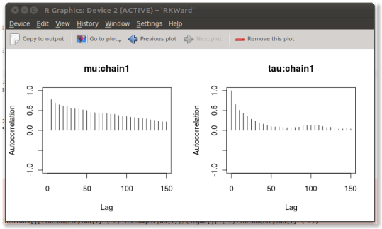
That looks terrible. Clearly this chain has not converged; mu looks terrible, in particular. You can do a smörgåsbord of convergence diagnostics through a wizard-like interface with codamenu(). This allows you, for example, to plot the autocorrelation of the chain:

Clearly, this won’t do.

A collapsed Gibbs sampler

Our chain exhibits poor convergence because mu and schoolmean are heavily correlated. This issue can be avoided by simply integrating out schoolmean, thus creating a collapsed Gibbs sampler. As this is a very simple model, this is straightforward:

model {
for(i in 1:N) {
thes[i] <- 1/(pow(sigma[i],2) + 1/itau)
schoolobs[i] ~ dnorm(mu,thes[i])
}

mu ~ dnorm(0,alpha)
alpha <- 1e-4
precisiontau <- .001
meantau <- 15
itau ~ dgamma(precisiontau, precisiontau*pow(meantau,2))
tau <- 1/sqrt(itau)
}

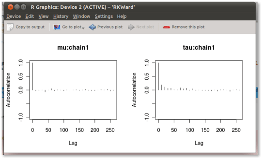
Running this new model, you can see that the autocorrelations are much better now:

Unfortunately, since we’ve removed schoolmean from the model through integration, we can’t get an estimate for the school means. You can, however, sample from the distribution of schoolmean in R using the conditional distribution of schoolmean given everything else (equation 5.17):

mu <- thesamps[[1]][,1]
tau <- thesamps[[1]][,2]

for(i in 1:1000) {
for(j in 1:8) {
meansi <- (sigma[j]^(-2)*schoolobs[j]+tau[i]^(-2)*mu[i])/(sigma[j]^(-2)+tau[i]^(-2))
stdsi  <- (sigma[j]^(-2)+tau[i]^(-2))^(-1/2)
R[i,j] <- rnorm(n = 1,mean=meansi,sd=stdsi)
}
}

You can then use functions like quantile and summary in R to obtain summary statistics for R. For me, this results in:

> summary(R)
V1               V2               V3                V4
Min.   :-8.608   Min.   :-6.836   Min.   :-30.082   Min.   :-13.263
1st Qu.: 5.686   1st Qu.: 4.842   1st Qu.:  4.078   1st Qu.:  4.630
Median : 8.551   Median : 7.597   Median :  7.260   Median :  7.789
Mean   : 9.162   Mean   : 7.842   Mean   :  7.138   Mean   :  7.741
3rd Qu.:12.471   3rd Qu.:10.984   3rd Qu.: 10.751   3rd Qu.: 11.128
Max.   :42.808   Max.   :28.813   Max.   : 28.604   Max.   : 30.446
V5                V6                V7               V8
Min.   :-11.165   Min.   :-27.112   Min.   :-6.713   Min.   :-14.780
1st Qu.:  3.489   1st Qu.:  4.153   1st Qu.: 5.717   1st Qu.:  4.735
Median :  6.743   Median :  7.365   Median : 8.656   Median :  7.908
Mean   :  6.532   Mean   :  7.139   Mean   : 9.079   Mean   :  8.047
3rd Qu.:  9.723   3rd Qu.: 10.526   3rd Qu.:12.171   3rd Qu.: 11.648
Max.   : 27.603   Max.   : 31.799   Max.   :31.714   Max.   : 33.428

You can see that compared to Table 5.3 in Gelman, the means are shrinked more towards the population mean as I have a proper prior on tau rather than a uniform one as in his example.