Our V4 Utah array died last week… and then it worked again this week. It’s pretty amazing that it’s still up and running after about 18 months. It’s gettting noisier, however, and increasingly what’s being recorded is mostly multi-unit activity (MUA).

To have any chance of detecting single units, it’s therefore quite important to denoise and optimally preprocess the signal. Here’s a rundown of how I do it. It took a lot of tinkering to get everything right, but I’m pretty satisfied with the results.

Of course, it’s important to avoid electrical interference, minimize line noise, use a Faraday cage, patch up some foil around leaky connections, etc. If you have the raw signals available, as opposed to only the waveform snippets, then you can do some more denoising offline. We sample every channel at 10 kHz. Here’s an example of one such channel, with a single good-sized spike on the right-hand side, as well as its time-changing power spectrum below.

As you can see, there’s only a little bit of line noise around 60Hz. More importantly, there’s no visible line noise harmonics around 180 Hz, 300 Hz, etc. The 60 Hz noise you can get rid of pretty easily by high-pass filtering, but the harmonics overlap the power spectrum of the spikes, so ideally you want to keep them to a minimum.

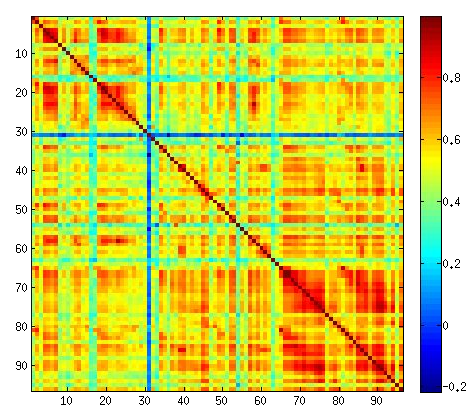
To detect spikes efficiently, it’s best to start by re-referencing the wideband channels. This will get rid of a lot of common noise, reward artifacts, etc. Take a look at the raw cross-correlations of the 96 channels:

Clearly most channels are highly correlated; that’s normal, since the electrodes only cover about 4 mm of cortex, and low frequency are strongly spatially correlated. Now let’s look at the cross-correlations after high-pass filtering the wideband data (using diff in Matlab):

Now we see a much different pattern. High-frequency information tends to be correlated in groups of 16 electrodes. The way the array is wired up, electrodes 1-16 are not necessarily close together on the array. However, they get sent together from the array to the amplifier on the same wire. That means that the correlation pattern that we’re seeing is probably common electrical noise.

Thus, I reference each electrode against the truncated mean of the group of 16 electrodes that it belongs to. I use the truncated mean (taking the mean of samples minus the largest and smallest 2) rather than the mean so that non-common high frequency information (ie spikes) don’t bleed across electrodes.

Next, I upsample the wideband data to 40kHz with cubic splines (csapi). I band pass filter with this snippet of code:

Wn = [500,6000]/40000*2;
[ha,hb] = ellip(2,.1,40,Wn);
upSampData = filtfilt(ha,hb,upSampData);

It’s pretty important, I’ve found, to use a filter which has a slow rolloff on either side of a passband, otherwise you get artifacts. After that, it’s pretty straightforward to detect spikes by thresholding. I use the median absolute deviation (mad) estimator for the noise power, and set the threshold to 4.4 times the standard deviation.

This gives me a bank of spikes which are aligned at their peak. Initially, I ran WaveClus directly on these snippets. However, it can be helpful to redo detection based on optimal filter based on the bank of spikes detected in the first round.

In theory optimal detection is straightforward. Assuming the noise of the signal is white, it simply involves convolving the signal with the template one wants to find. However it’s a bad idea to whiten the signal after upsampling.

So what I do instead is this. I take the mean spike from the first round, and filter it twice with a pseudo-noise-whitening matrix. I say pseudo, because if you take noise snippets and compute the covariance of the noise, you’ll find that it’s very poorly conditioned. If E is the noise covariance matrix, I add 5*eye(128)+.2*diag(((1:128)-56).^2) before taking the eigendecomposition to form a whitening matrix. 56 is the time sample where the peak of the waveform is located. Adding a quadratic term to the diagonal of the covariance matrix ensures that the whitening filter only acts on the area of the spike that contains the peak. Here’s the spike on the left, the (pseudo) whitening matrix in the middle, and the spike after double-whitening. You can see that unlike with a true whitening filter, the double-whitened spike acts locally.

Redetection can be quite helpful for spikes which who are just on the edge of the threshold. Here’s the distribution of the (negative of) the band-pass signal for one electrode. You can see that there’s a pedestal like feature on the right which indicates that there’s some spikes there. If you look only at the local maxima of the signal (right plot), however, you’ll notice that a threshold (shown in blue) can’t separate this activity from the noise very well.

Once you optimally filter, however, you get the distributions below. Notice that the optimal filter moves the spikes out of the background noise distribution, so that it can quite clearly be separated using a simple threshold. After this, all that is left to do is sort the spike snippets in WaveClus.